Classifying Fashion-MNIST using MLP in Pytorch
Fashion-MNIST is a dataset of Zalando’s article images—consisting of a training set of 60,000 examples and a test set of 10,000 examples. Each example is a 28x28 grayscale image, associated with a label from 10 classes.
import torch
from torchvision import datasets, transforms
import helper

# Define a transform to normalize the data
transform = transforms.Compose([transforms.ToTensor()])

#transforms.ToTensor() convert our image to a tensor
#transforms.Normalize() will normalizae our image with provided mean and sd values

# Download and load training data

trainset = datasets.FashionMNIST('./data',download=True, train= True, transform=transform)
trainloader = torch.utils.data.DataLoader(trainset, batch_size= 64, shuffle=True)

# Download and load test data
testset = datasets.FashionMNIST('./data',download=True, train= False, transform=transform)
testloader = torch.utils.data.DataLoader(testset, batch_size= 64, shuffle=True)
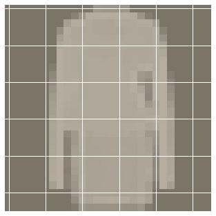
Lets check one of the images
image, label = next(iter(trainloader))
helper.imshow(image[0,:])
image.view(image.shape[0],-1).shape
torch.Size([64, 784])
Building the network
As each image is 28x28 which is a total of 784 pixels, and there are 10 classes. Lets use 3 hidden layers and ReLU activation function to the network
#Network parameters

input_size = 784 #i.e 28*28*1
hidden_size = [256,128,64]
out_size = 10
Train the network
Here we will define loss function (to calculate the loss nn.CrossEntropyLoss ) and optimizer to update our parameters or weights (typically optim.SGD or optim.Adam).
- Make a forward pass through the network to get the logits.
- Use the logits to calculate the loss.
- Perform a backward pass through the network with loss.backward() to calculate the gradients.
- Take a step with the optimizer to update the weights
from torch import nn
from torch.nn import NLLLoss
from torch.optim import SGD

model = nn.Sequential(
nn.Linear(input_size,hidden_size[0]),
nn.ReLU(),
nn.Linear(hidden_size[0],hidden_size[1]),
nn.ReLU(),
nn.Linear(hidden_size[1],hidden_size[2]),
nn.ReLU(),
nn.Linear(hidden_size[2],out_size),
nn.LogSoftmax(dim=1)
)

criterion = NLLLoss()
optimizer = SGD(model.parameters(),lr=0.001)
print(model)
Sequential(
  (0): Linear(in_features=784, out_features=256, bias=True)
  (1): ReLU()
  (2): Linear(in_features=256, out_features=128, bias=True)
  (3): ReLU()
  (4): Linear(in_features=128, out_features=64, bias=True)
  (5): ReLU()
  (6): Linear(in_features=64, out_features=10, bias=True)
  (7): LogSoftmax()
)
epochs =10

for e in range(epochs):
  running_loss = 0
  for images, labels in trainloader:

    #Flatten the image into a 784 long vector

    images = images.view(images.shape[0],-1) #sqash the image in to 784*1 vector

    #reset the default gradients
    optimizer.zero_grad()

    # forward pass
    output = model(images)
    loss = criterion(output,labels)

    #backward pass calculate the gradients for loss
    loss.backward()

    # update the parameters
    optimizer.step()

    running_loss = running_loss+loss.item()
  else:
    print(f"Training loss: {running_loss/len(trainloader)}")
Training loss: 2.2909004207867296
Training loss: 2.260512700721399
Training loss: 2.2062994226463823
Training loss: 2.106043025120489
Training loss: 1.9362352307417245
Training loss: 1.6625972527430763
Training loss: 1.3871929200727549
Training loss: 1.2008064909657437
Training loss: 1.0784652017072829
Training loss: 0.9925383474908149
Testing the network
%matplotlib inline
%config InlineBackend.figure_format = 'retina'
# Test out your network!
dataiter = iter(testloader)
images, labels = dataiter.next()
img = images[0]
# Convert 2D image to 1D vector
img = img.resize_(1, 784)
#turn off the gradients
with torch.no_grad():
logps = model(img)
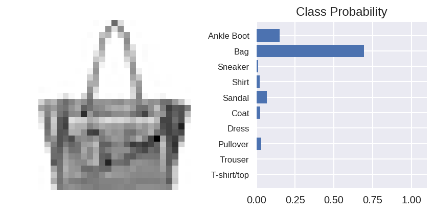
# TODO: Calculate the class probabilities (softmax) for img
ps = torch.exp(logps)
# Plot the image and probabilities
helper.view_classify(img.resize_(1, 28, 28), ps, version='Fashion')