Introduction Deep Convolutional Neural Networks
Problem with traditional Neural Networks or Multi Layer Perceptrons
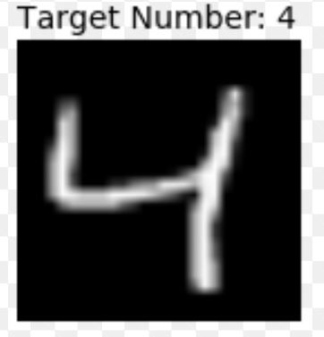
Every image is an arrangement of dots (a pixel) arranged in a special order. If you change the order or color of a pixel, the image would change as well. Let us take an example. Let us say, you wanted to store and read an image with a number 4 written on it.The machine will basically break this image into a matrix of pixels and store the color code for each pixel at the representative location.
here is how machine looks at a hand written image.
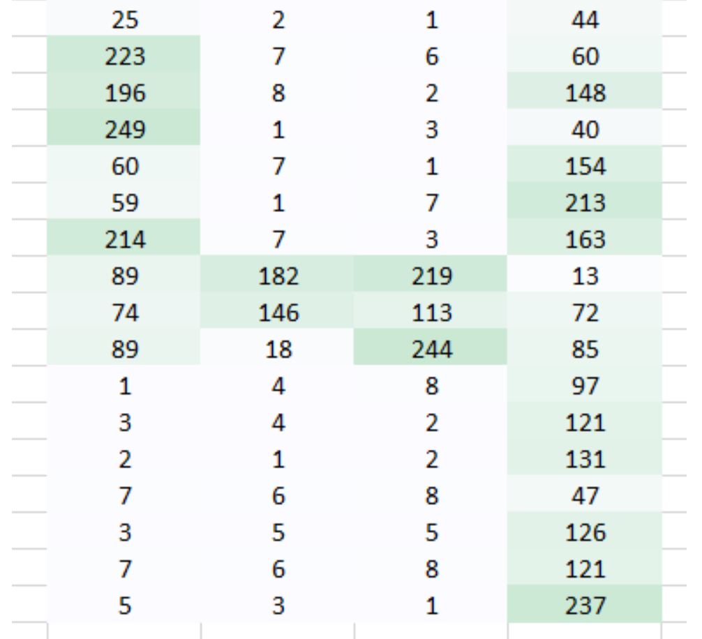
A fully connected network would take this image as an array by flattening it and considering pixel values as features to predict the number in image.
The problem with this approach are
- Not enough computational power
As machine see an image as a matrix of numbers where each number corresponds to the pixel value. An image of size 256 x 256 x 3 is a matrix with 3 layers (RGB) where each layer contains 256 x 256 values.
When we flatten these values in to a vector and feed into a network we are feeding 196,608 inputs.If, for example, we have 1,000 hidden units in our first hidden layer, there would be approximately 196 million parameters or weights for us to train which is infeasible.
- Local Features Loss
With images, you normally do want to preserve the local features. What we mean by this is if you want to classify a cat, we would like to preserve the key features such as the face or ears of the cat. However, by flattening the matrix, we have removed all those local features which is not a good approach. Even with these obstacles, people have invented a new way to solve these problems with the technique which is known as convolution.
Convolution of Images
In CNN, We can take the input image, define a weight matrix and the input is convolved to extract specific features from the image without losing the information about its spatial arrangement.
Another great benefit this approach has is that it reduces the number of parameters from the image. As you saw above the convolved images had lesser pixels as compared to the original image. This dramatically reduces the number of parameters we need to train for the network.
Convolution is a mathematical operation that takes two inputs:
- An image matrix (volume) of dimension (h x w x d)
- A filter (f_h x f_w x d) and outputs a volume of dimension (h — f_h + 1) x (w — f_w + 1) x 1.
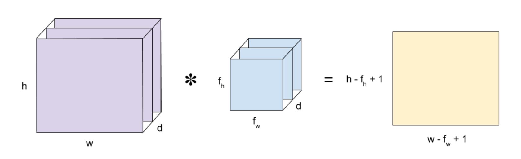
A filter will slide over our original image by 1 pixel (also called ‘stride’) and for every position, we compute element wise multiplication (between the two matrices) and add the multiplication outputs to get the final integer which forms a single element. computing the dot product is called the ‘Convolved Feature’ or ‘Activation Map’ or the ‘Feature Map‘. It is important to note that filters acts as feature detectors from the original input image.
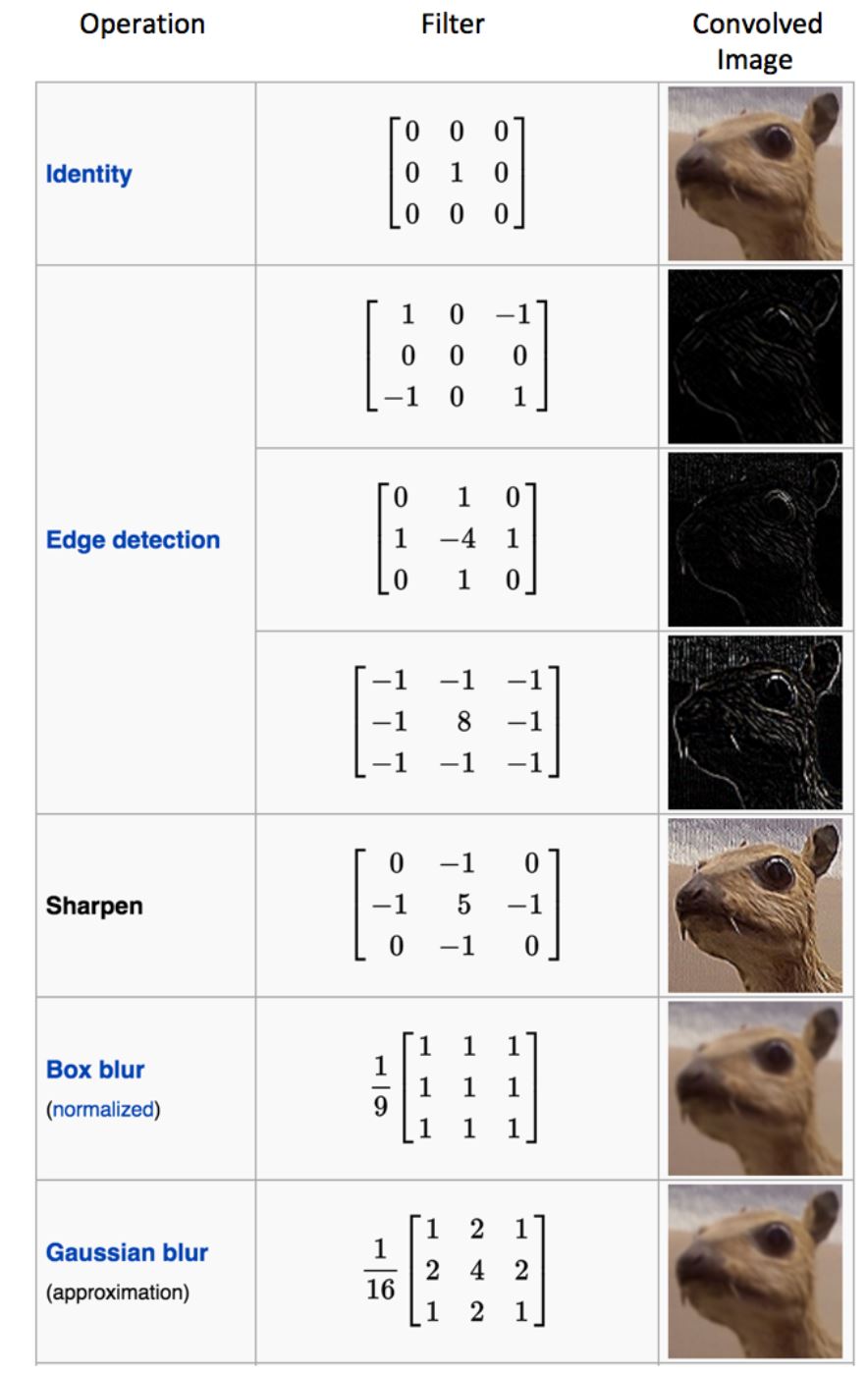
In the table below, we can see the effects of convolution of the above image with different filters. As shown, we can perform operations such as Edge Detection, Sharpen and Blur just by changing the numeric values of our filter matrix before the convolution operation.
Convolution Layer
A convolution layer is composed of n_f filters of the same size and depth of a original image. For each filter, we convolve it with the input volume to obtain n_f outputs.Finally, those n_f outputs is stacked together into a (h — f_h + 1) x (w — f_w + 1) x n_f volume.
Performing convolutions on images instead of connecting each pixel to the neural network units has two main advantages:
- Reduces the number of parameters we need to learn. As we are extracting features from a filter rather than looking at whole image number of parameters involved significantly reduces. (filter size is lot smaller than the input image)
- Preserves locality. We don’t have to flatten the image matrix into a vector, thus the relative positions of the image pixels are preserved. Take a cat image for example. The information that makes up a cat includes the relative positions of its eyes, nose, and fluffy ears. We lose that insight if we represent the image as one long string of numbers.
The size of the Feature Map (Convolved Feature) is controlled by three parameters that we need to decide before the convolution step is performed:
- Depth: Depth corresponds to the number of filters we use for the convolution operation.
- Stride: Stride is the number of pixels by which we slide our filter matrix over the input matrix. When the stride is 1 then we move the filters one pixel at a time.
- Zero-padding: This helps us to preserve the size of the input image. If a single zero padding is added, a single stride filter movement would retain the size of the original image. where as a valid padding drops the part of image where filter didn’t fit.
Introducing Non Linearity (ReLU)
An additional operation called ReLU has been used after every Convolution. ReLU stands for Rectified Linear Unit and is a non-linear operation. Its output is given by:
ouput = Max(zero, Input)
The purpose of ReLU is to introduce non-linearity in our ConvNet, since most of the real-world data we would want our ConvNet to learn would be non-linear (Convolution is a linear operation – element wise matrix multiplication and addition, so we account for non-linearity by introducing a non-linear function like ReLU).
Other non linear functions such as tanh or sigmoid can also be used instead of ReLU, but ReLU has been found to perform better in most situations.
The Pooling Step
Spatial Pooling (also called subsampling or downsampling) reduces the dimensionality of each feature map but retains the most important information. Spatial Pooling can be of different types: Max, Average, Sum etc.
In case of Max Pooling, we define a spatial neighborhood (for example, a 2×2 window) and take the largest element from the rectified feature map within that window. Instead of taking the largest element we could also take the average (Average Pooling) or sum of all elements in that window. In practice, Max Pooling has been shown to work better.
- Makes the input representations (feature dimension) smaller and more manageable
- Reduces the number of parameters and computations in the network, therefore, controlling overfitting.

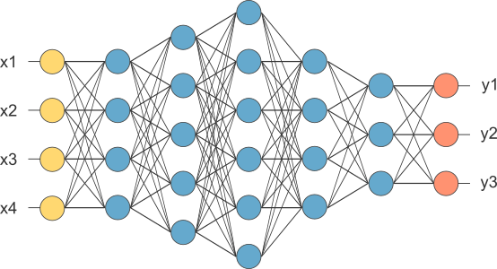
Fully Connected Layer
The term “Fully Connected” implies that every neuron in the previous layer is connected to every neuron on the next layer. We flattened our matrix into vector and feed it into a fully connected layer like neural network. We have this layer in order to add non-linearity to our data. If to give an example of a human face, the convolutional layer might be able to identify features like faces, nose, ears, and etc. However, they do not know the position or where these features should be. With the fully connected layers, we combined these features together to create a more complex model that could give the network more prediction power as to where these features should be located in order to classify it as human.
The sum of output probabilities from the Fully Connected Layer is 1. This is ensured by using the Softmax as the activation function in the output layer of the Fully Connected Layer. The Softmax function takes a vector of arbitrary real-valued scores and squashes it to a vector of values between zero and one that sum to one.
Backpropagation
While forward propagation(Convolution + pooling + fc layer) carries information about the input x through successive layers of neurons to approximate y with ŷ, backpropagation carries information about the cost (error) C backwards through the layers in reverse and, with the overarching aim of reducing cost, adjusts neuron parameters (weights) throughout the network.
In Backpropagation we calculate the gradients of the error with respect to all weights in the network and use gradient descent to update all filter values / weights and parameter values to minimize the output error.
“Backpropagation is the process of calculating the gradients of functions through the recursive application of the chain rule.”
Backpropagation sends our network’s error back through our network by taking partial derivatives of the loss function. Basically, it’s deciding how much the algorithm will need to change it’s weights by in order to compensate for any bad predictions it just made on the forward pass. At each node in the network, it calculates the error with respect to the weights